Introduction
Compounding is one of the most powerful financial concepts that helps grow investments exponentially over time. Whether you’re calculating compound interest, investment growth, or savings accumulation, Excel provides multiple ways to implement compounding formulas.
In this comprehensive guide, we will cover everything you need to know about compounding formula in Excel, including:
- Basic compound interest formula
- Using Excel functions like FV, PV, RATE, and NPER
- Handling regular deposits and withdrawals
- Different scenarios where compounding is useful
- Using tables and dynamic formulas for better visualization
By the end of this article, you’ll be able to apply these formulas to real-world financial scenarios effectively.
1. Understanding the Compound Interest Formula
Before diving into Excel, let’s first understand the basic compound interest formula:
A = P x (1 + r / n)nt
Where:
- A = Final amount after compounding
- P = Principal (initial investment)
- r = Annual interest rate (as a decimal)
- n = Number of times interest is compounded per year
- t = Number of years
This formula helps determine how investments grow over time when interest is compounded periodically.
2. Basic Compound Interest Calculation in Excel
Method 1: Using a Direct Formula
You can use a simple Excel formula to calculate compound interest:
=A2*(1+B2/C2)^(C2*D2)
Where:
- A2 = Principal amount
- B2 = Interest rate
- C2 = Number of times compounded per year
- D2 = Number of years
Example:
Assume an investment of $10,000 with an 8% annual interest rate, compounded quarterly for 5 years.

Final result: $14,859
3. Using Excel Functions for Compound Interest
Excel provides built-in financial functions that make compound interest calculations easier.
Method 2: Using the FV (Future Value) Function
FV(rate, nper, pmt, pv, type) is a built-in Excel function to calculate future value.
Formula:
=FV(rate, nper, pmt, pv, type)
Where:
- rate = Interest rate per period
- nper = Total number of periods
- pmt = Periodic payment (use 0 for a lump sum investment)
- pv = Present value (initial investment, enter as a negative value)
- type = 0 (end of period) or 1 (beginning of period)
Example:
=FV(8%/4, 4*5, 0, -10000, 0)
This will return $14,859.

Method 3: Using PV, RATE, and NPER for Reverse Calculations
These functions are useful when you need to work backwards from a future value to determine the present value, interest rate, or number of periods required.
1. PV (Present Value) Function
Formula:
=PV(rate, nper, pmt, fv, type)
This function calculates the initial investment required to reach a future amount under given conditions.
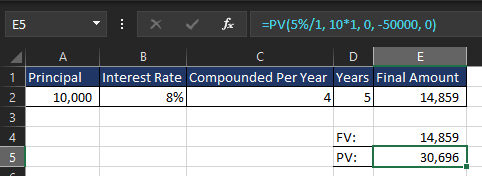
Example: If you want $50,000 in 10 years with an annual interest rate of 5%, compounded yearly:
=PV(5%/1, 10*1, 0, -50000, 0)
This will return $30,696, meaning you need to invest this amount today.
2. RATE (Interest Rate) Function
Formula:
=RATE(nper, pmt, pv, fv, type)
This function helps determine the interest rate required to reach a financial goal.
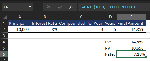
Example: If you invest $10,000 for 10 years and expect to reach $20,000, use:
=RATE(10, 0, -10000, 20000, 0)
This will return 7.18%, meaning you need this annual interest rate to double your investment in 10 years.
3. NPER (Number of Periods) Function
Formula:
=NPER(rate, pmt, pv, fv, type)
This function calculates how long it takes to reach a financial goal under a given interest rate.
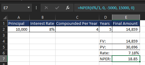
Example: If you invest $5,000 with an annual interest rate of 6% and want to reach $15,000:
=NPER(6%/1, 0, -5000, 15000, 0)
This will return 18.85 years, meaning it will take that long to reach $15,000.
4. Compound Interest with Regular Deposits (Recurring Investments)
Many investors make regular deposits instead of a one-time investment. The formula changes slightly:

Where:
- D = Regular deposit per period
Example Using Excel:
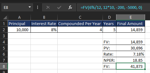
If you invest $200 monthly into an account with an annual 6% interest rate, compounded monthly for 10 years, use:
=FV(6%/12, 12*10, -200, -5000, 0)
This considers both the initial investment and monthly contributions.
Final amount: $41,873
5. Different Scenarios Where Compounding is Useful
1. Retirement Planning
Planning for retirement is one of the most common uses of compounding in Excel. By using the right formulas, you can determine how much you need to save each month to reach a desired retirement fund. This helps individuals plan their financial future and make informed decisions about their savings strategy.
How Compounding Helps in Retirement Planning
When saving for retirement, your money grows over time through compound interest. The earlier you start, the more you benefit from compounding because interest is earned not only on your original contributions but also on the accumulated interest over time.
To estimate how much you need to save every month, you can use Excel’s FV (Future Value) function, which calculates the value of an investment after a series of periodic deposits with compound interest.
Formula for Calculating Retirement Savings in Excel
The FV function formula in Excel is:
=FV(rate, nper, pmt, pv, type)
Where:
- rate = Interest rate per period (annual rate divided by number of periods per year)
- nper = Total number of periods (years × periods per year)
- pmt = Payment made each period (monthly savings amount)
- pv = Present value or starting amount (use 0 if starting fresh)
- type = 0 (end of the period) or 1 (beginning of the period)
Example: How Much to Save Monthly for Retirement?
Correct Solution Using Excel:
To find how much John needs to save each month, use the PMT function. The formula will look like this:
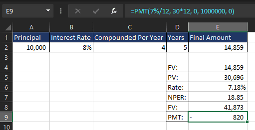
=PMT(7%/12, 30*12, 0, 1000000, 0)
Where:
- 7%/12 is the monthly interest rate (7% annual divided by 12 months).
- 30*12 is the total number of periods (30 years * 12 months).
- 0 is the present value (no initial investment, so it’s 0).
- 1000000 is the future value (the amount John wants to have at the end).
- 0 specifies that payments are made at the end of each period (the end of each month).
When you use the formula in Excel, the result will be -820 (the negative sign indicates an outflow of money, which makes sense for monthly savings). You can simply ignore the negative sign and say that John needs to save $820 each month.
What If John Starts Later?
If John delays saving by 10 years and starts at age 40, the number of periods reduces to 20 years (20 years * 12 months). The formula will be:
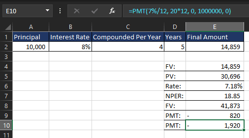
=PMT(7%/12, 20*12, 0, 1000000, 0)
This returns a monthly contribution of -1,920. Again, the negative sign means it’s an outflow, so John needs to save $1,920 each month if he starts at age 40.
Key Takeaways:
- If John saves for 30 years, he needs to save $820 per month.
- If he starts 10 years later, at age 40, he will need to save $1,920 per month.
2. Loan Repayments with Compounding in Excel
Loans, such as mortgages, student loans, or car loans, accrue interest over time, and making extra payments can significantly reduce the total interest paid and shorten the repayment period. Using Excel’s loan-related functions, you can analyze how different repayment strategies affect your debt.
How Compounding Affects Loan Repayments
When you take out a loan, the lender charges interest on the remaining balance. Each payment you make consists of:
- Principal – The amount that goes toward reducing the loan balance.
- Interest – The cost of borrowing, calculated based on the outstanding principal.
If you only make the required minimum payments, you could end up paying much more in interest over the loan term. However, making extra payments reduces the principal faster, which in turn reduces the interest charged.
Formula for Loan Repayments in Excel
The PMT (Payment) function in Excel calculates the required monthly payment for a loan:
=PMT(rate, nper, pv, fv, type)
Where:
- rate = Interest rate per period (annual rate divided by 12 for monthly payments)
- nper = Total number of periods (years × 12)
- pv = Loan amount (present value)
- fv = Future value (use 0 for full repayment)
- type = 0 (end of period) or 1 (beginning of period)
Example: Calculating Monthly Loan Payments
Scenario:
Emma takes out a $200,000 mortgage with a 5% annual interest rate for 30 years. She wants to know her required monthly payment.
Solution Using Excel:
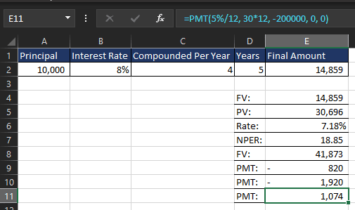
=PMT(5%/12, 30*12, -200000, 0, 0)
Where:
- 5%/12 → Monthly interest rate
- 30*12 → Total payments (30 years × 12 months)
- -200000 → Loan amount (negative because it’s a liability)
- 0 → No remaining balance at the end of the loan
- 0 → Payments made at the end of each month
Excel returns a monthly payment of $1,074.
How Extra Payments Reduce Interest
What if Emma adds an extra $200 per month toward the loan principal?
Instead of paying $1,074, she pays $1,274 per month.
To see how this impacts her loan term, we use the NPER (Number of Periods) function:
=NPER(5%/12, -1274, 200000, 0, 0)
After running the formula, it should give you the result in months, and then you can divide the number of months by 12 to get the number of years.
The formula returns approximately 255 months, which is about 21.25 years.
So, by making an extra $200 payment per month, Emma will pay off her loan in 21 years, saving approximately 9 years off her loan term compared to the original 30-year term.
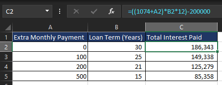
Comparing Different Repayment Strategies

This table clearly shows how even small extra payments can save years on a loan and reduce the total interest paid.
To calculate the loan term, you can use the following formula:
=NPER(5%/12, -1074-A2, 200000, 0, 0)/12
To calculate the total interest paid on a loan, you can use the following formula:
= (Monthly Payment x Loan Term) – Loan Value
In our table this formula would be:
=((1074+A2)*I2*12)-200000
Key Takeaways for Loan Repayments in Excel
- Total Interest Paid Formula – The total interest paid over a loan’s lifetime is calculated as:
Total Interest=(Monthly Payment×Total Months)−Loan Principal
This helps borrowers understand the real cost of their loan.
- Extra Payments Save Money – Making additional payments toward the principal reduces both the loan term and total interest paid. Even small extra payments can lead to significant savings.
- Earlier Payments Have a Bigger Impact – The sooner you make extra payments, the more you save on interest. Interest accrues over time, so early reductions in principal reduce long-term costs.
- NPER Function Determines New Loan Term – When making extra payments, the NPER function in Excel can calculate how much sooner the loan will be paid off.
- Comparing Repayment Strategies is Crucial – Running different scenarios in Excel helps borrowers choose the best strategy for faster payoff and minimizing interest.
- Higher Interest Loans Benefit Even More from Extra Payments – The higher the interest rate, the greater the impact of extra payments on total savings.
3. Business Growth Forecasting Using Compounding in Excel
Businesses use compounding formulas to estimate future revenue growth, taking into account factors like reinvestment, interest, and increasing returns. Excel provides powerful financial functions to model different growth scenarios, helping businesses strategize their expansion effectively.
How Compounding Affects Business Growth
Compounding plays a crucial role in business growth when:
- Profits are reinvested – Earnings are reinvested to generate more revenue over time.
- Interest or returns accumulate – If the company has savings or investments, they compound over time.
- Customer base grows – A steady increase in customers leads to higher revenue each year.
By using compounding formulas in Excel, businesses can predict future revenue, evaluate investment decisions, and plan long-term strategies.
Formula for Business Growth in Excel
To calculate future revenue growth, businesses use the compound growth formula:
FV = PV × (1 + r)t
Where:
- FV = Future value (projected revenue)
- PV = Present value (current revenue)
- r = Growth rate per period (as a decimal)
- t = Number of periods (years)
In Excel, this formula can be written as:
=A2*(1+B2)^C2
Where:
- A2 = Current revenue
- B2 = Growth rate
- C2 = Number of years
Example: Predicting Future Revenue
Scenario:
A startup currently generates $100,000 in annual revenue. The company expects to grow at a 10% annual rate by reinvesting profits.
Solution Using Excel:
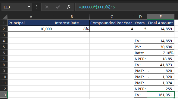
=100000*(1+10%)^5
This returns $161,051, meaning in 5 years, revenue is expected to grow from $100,000 to $161,051.
Using the FV Function for Growth Projections
Instead of a manual formula, you can use Excel’s FV (Future Value) function:
=FV(rate, nper, pmt, pv, type)
Where:
- rate = Growth rate per period
- nper = Number of periods (years)
- pmt = Additional contributions per period (use 0 if none)
- pv = Initial revenue (entered as a negative value)
- type = 0 (end of period) or 1 (beginning of period)
Example:
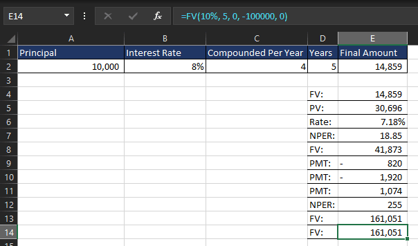
=FV(10%, 5, 0, -100000, 0)
This also returns $161,051.
What If the Company Reinvests Profits?
If the company reinvests $20,000 per year from profits into expansion, we adjust the FV formula:
=FV(10%, 5, -20000, -100000, 0)
Now, the projected revenue is $283,153 after 5 years.
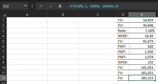
By reinvesting $20,000 annually, the company can nearly double its revenue compared to passive growth.
Comparing Different Growth Strategies


This table shows how higher growth rates and reinvestments significantly impact revenue.
Key Takeaways for Business Growth Forecasting in Excel
- Use Compound Growth Formulas – Model long-term revenue projections.
- Leverage the FV Function – Easily calculate future revenue based on different growth rates.
- Analyze Reinvestment Impact – Adjust formulas to include additional contributions.
- Compare Strategies – Test different growth rates and reinvestment levels to optimize business expansion.
4. College Savings
Parents and students can calculate how much to invest today to afford future education expenses. This helps in ensuring adequate financial preparation for tuition and other costs. With the rising cost of education, early planning is key to minimizing financial strain when it’s time to pay for college or university. By investing in the right savings plan and using compounding to grow their money, families can ensure they’re financially prepared.
How Compounding Affects College Savings
Compounding plays a crucial role in saving for college, as it allows money to grow over time, making it easier to reach the required amount for tuition and other expenses. Compounding works in the following ways:
- Interest Accumulation: The money you invest today earns interest over time, which then earns interest on itself.
- Regular Contributions: By contributing to a savings account regularly, each new deposit also benefits from compounding growth.
- Time Horizon: The longer the time frame before the education expenses are needed, the more time your money has to grow and compound.
By understanding how compounding works and utilizing the right savings vehicle, parents can grow their initial investment into a significant amount to cover future education costs.
Formula for College Savings in Excel
To calculate how much to save for future college expenses, the Future Value (FV) formula is used. The formula calculates how much your current investment will grow to in the future based on the rate of return and the time you leave it to grow.
The formula for future value is:
FV = PV × (1 + r)t
Where:
- FV = Future value (the amount needed for college)
- PV = Present value (the current amount invested)
- r = Growth rate per period (as a decimal, e.g., 5% = 0.05)
- t = Number of periods (years until college starts)
In Excel, you can use this formula as follows:
=A2*(1+B2)^C2
Where:
- A2 = Current investment
- B2 = Growth rate (annual return rate)
- C2 = Number of years
Example: Predicting Future College Costs
Scenario: You estimate that the total cost for college education in 10 years will be $100,000. To reach that goal, you want to calculate how much you need to invest today, assuming an annual return of 6%.
Solution Using Excel: Let’s say you want to find out how much to invest today to reach that $100,000 in 10 years with a 6% return rate.
The formula would be:
=100000/(1+6%)^10
This will return a value of $55,839, meaning you would need to invest $55,839 today to have $100,000 in 10 years, assuming a 6% return rate.
Using the FV Function for College Savings
Instead of manually calculating with the compound growth formula, you can use Excel’s FV (Future Value) function. This function helps simplify the calculation of future savings based on regular contributions.
The formula for FV in Excel is:
=FV(rate, nper, pmt, pv, type)
Where:
- rate = Growth rate per period (annual return rate)
- nper = Number of periods (years until college)
- pmt = Additional contributions per period (use 0 if none)
- pv = Initial investment (entered as a negative value)
- type = 0 (end of period) or 1 (beginning of period)
Example:
If you invest $5,000 today with no additional contributions and a 6% return over 10 years, the formula would be:
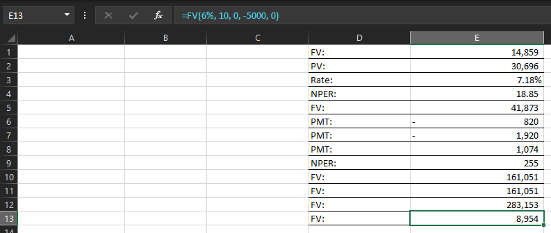
=FV(6%, 10, 0, -5000, 0)
This returns $8,954, meaning your $5,000 investment would grow to $8,954 in 10 years at a 6% annual return.
What If You Contribute Regularly?
If you want to make monthly contributions to your college savings, you can adjust the FV formula to include periodic payments.
Scenario: You plan to save $300 per month for the next 10 years, along with an initial investment of $5,000. Your annual return rate is 6%.
The formula in Excel would be:
=FV(6%/12, 10*12, -300, -5000, 0)
This returns $55,261, meaning after 10 years of monthly contributions of $300, along with your initial investment, you’ll have a total of $55,261.
Comparing Different Saving Scenarios
You can compare different saving strategies using the following table, which compares different growth rates and investment strategies:

Key Takeaways for College Savings in Excel
- Understand Compounding – The longer you save, the more your money will grow.
- Use the FV Function – Quickly calculate how much your savings will be worth in the future with regular contributions.
- Include Monthly Contributions – Regular contributions can help boost your savings significantly over time.
- Test Different Scenarios – Experiment with different growth rates, time horizons, and contribution levels to see how they impact your total savings.
5. Inflation-Adjusted Growth
When investing for long-term growth, it’s crucial to consider inflation as it erodes purchasing power over time. While nominal returns (the raw return on investment) show how much your investment grows, real returns take inflation into account to reflect the actual value increase of your money. Understanding inflation-adjusted growth allows investors to assess their true returns, ensuring that they don’t just beat inflation but also grow their wealth in real terms.
How Inflation Affects Investment Growth
Inflation can diminish the real value of your investments by decreasing the purchasing power of the future value of money. Here’s how compounding interacts with inflation:
- Nominal Growth: The return on your investment without accounting for inflation.
- Real Growth: The return after factoring in inflation, reflecting the true increase in purchasing power.
- Purchasing Power: As prices rise over time, the same amount of money will buy fewer goods and services. Therefore, it’s important to calculate how much your investment needs to grow in real terms to maintain or increase your standard of living.
To accurately assess the growth of your investment, you need to consider both the nominal return and the inflation rate, as the latter reduces the value of future returns.
Formula for Inflation-Adjusted Growth in Excel
To calculate inflation-adjusted growth, you need to factor in the real return. The formula to adjust for inflation is:

Where:
- Nominal Return = The annual return of your investment (expressed as a decimal).
- Inflation Rate = The annual inflation rate (also expressed as a decimal).
In Excel, you can calculate this using:
=(1 + B2)/(1 + C2) – 1
Where:
- B2 = Nominal return rate
- C2 = Inflation rate
Example: Adjusting Investment Growth for Inflation
Scenario: You are investing in a fund that offers a 7% return per year. However, the inflation rate is 3% annually. You want to know your real return after factoring in inflation over a 10-year period.
Solution Using Excel: First, calculate the real return by using the inflation-adjusted formula:
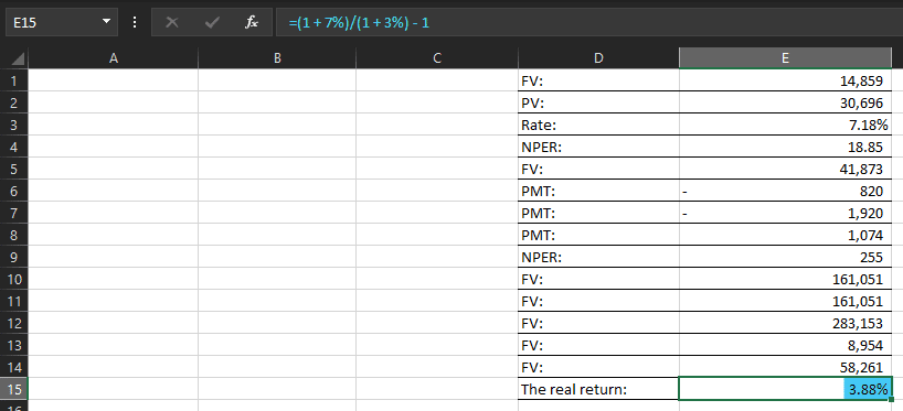
=(1 + 7%)/(1 + 3%) – 1
This will return a real return of 3.88%. This means that after accounting for inflation, your money is growing at 3.88% per year in real terms, not the nominal 7%.
Using the FV Function for Inflation-Adjusted Growth
After adjusting for inflation, you can project the future value of your investment using the Future Value (FV) function in Excel. This allows you to calculate how much your money will grow in real terms over time, considering both the nominal return and inflation.
The formula for FV is:
=FV(rate, nper, pmt, pv, type)
Where:
- rate = Nominal growth rate (inflation-adjusted rate)
- nper = Number of periods (years)
- pmt = Periodic payments (if any)
- pv = Present value (initial investment)
- type = 0 (end of period) or 1 (beginning of period)
Example: If you invest $10,000 today with a nominal return of 7% and an inflation rate of 3%, you can adjust for inflation and calculate how much your investment will grow in real terms over 10 years.
The formula for this would be:
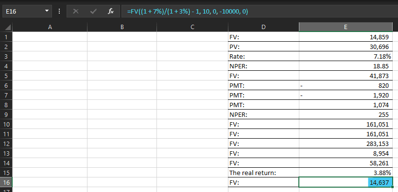
=FV((1 + 7%)/(1 + 3%) – 1, 10, 0, -10000, 0)
This returns $14,637 in real terms. After accounting for inflation, your $10,000 investment will grow to $14,637 in real terms over 10 years.
What If You Contribute Regularly?
If you plan to make regular contributions to your investment, you need to adjust for inflation in the same way. Monthly contributions can significantly impact the final amount, especially when factoring in inflation.
Scenario: You invest $200 per month in a fund that earns a 7% annual return, but inflation is 3% per year. Additionally, you start with an initial investment of $10,000. How much will your total investment be worth in today’s money after 10 years?
The formula would be:
=FV((((1+7%)/(1+3%))-1)/12, 10*12, -200, -10000, 0)
Breakdown of the Formula:
- ((1+7%)/(1+3%))-1 → Adjusts the 7% nominal return to reflect real (inflation-adjusted) growth.
- /12 → Converts the annual real return into a monthly rate.
- 10*12 → Total number of months (10 years × 12 months).
- -200 → Monthly contribution (negative because it’s an outflow).
- -10000 → Initial investment (negative because it’s an outflow).
- 0 → Payments are made at the end of each month.
Final Answer:
After 10 years, your investment will be worth $44,006 in today’s money after adjusting for inflation.
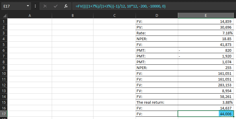
This shows the real purchasing power of your savings, helping you make informed financial decisions.
Comparing Different Inflation Scenarios
You can also compare how different inflation rates impact your investment growth. Here’s a table showing various inflation rates, nominal returns, and the resulting real returns over 10 years:

This table shows how higher inflation rates can reduce the real return, which impacts the future value of your investments.
Key Takeaways for Inflation-Adjusted Growth in Excel
- Understand the Impact of Inflation – Inflation erodes purchasing power, so it’s important to calculate real returns to gauge actual growth.
- Adjust for Inflation – Use the formula to calculate the real return after adjusting for inflation.
- Use the FV Function – Calculate how your investment will grow in real terms, including periodic contributions.
- Compare Scenarios – Test different inflation rates and nominal returns to see how they affect future investment growth.
By factoring in inflation and using Excel’s powerful financial functions, you can make informed investment decisions and ensure that your money grows in real terms, helping you preserve purchasing power and achieve your financial goals.
Conclusion
Excel is an incredibly powerful tool for managing your finances, and when it comes to compound interest and growth, it offers unparalleled capabilities to help you plan, predict, and optimize your financial future. Whether you’re tracking personal investments, forecasting business growth, planning for major purchases like college tuition, or adjusting for inflation, understanding and applying the compounding formula in Excel is a game-changer.
In today’s world, mastering these compounding techniques is no longer just for financial experts or large corporations. With the right knowledge, you can harness Excel’s functions to make smarter decisions in every area of your financial life. Imagine being able to accurately predict how your savings will grow over time, or how your business’s revenue could expand under different scenarios. You could estimate how much you need to save today to meet future educational expenses or how to adjust for inflation to maintain your purchasing power in the long run.
By using Excel’s built-in functions such as FV, PMT, and other financial formulas, you’re equipped to tackle a variety of financial calculations with ease. You can experiment with different growth rates, reinvestment strategies, or inflation adjustments to see the full potential of your financial planning. These techniques empower you to take control of your money and ensure that you’re not only growing your wealth but doing so in the smartest, most efficient way possible.
As you move forward with your financial planning, remember that the key to success is consistency. Whether you’re tracking your investments, saving for retirement, or planning for major life expenses, using compounding principles in Excel will help you better understand the long-term implications of your decisions and ensure you’re on the right path to financial security.
Now that you have a complete understanding of how compounding works in Excel, it’s time to put this knowledge into action. Don’t just read about these formulas—try applying them to your own financial situation. With each new calculation, you’ll gain more insight into how small decisions today can lead to substantial growth tomorrow.
The world of finance can feel daunting, but with the right tools and knowledge, it becomes much more manageable. Let Excel be your guide, and take control of your financial destiny with confidence. Try out these formulas, experiment with different variables, and watch how your wealth can grow exponentially. Mastering compounding in Excel isn’t just about crunching numbers; it’s about gaining a deeper understanding of your financial future and making informed decisions that will set you up for long-term success. So, take the first step today and start using these powerful formulas in Excel to create a brighter, more secure
